Generating Mock Posterior Estimates

Introduction

In this tutorial, we will generate mock posterior estimates similar to those used in [1] using per-defined CLIs in GWKokab. Primary source mass and mass ratio of BBH are jointly parameterized by Powerlaw Primary Mass Ratio.

\[ p(m_1, q\mid \alpha,\beta,m_\mathrm{min},m_\mathrm{max}) \propto m_1^{-\alpha} q^{\beta} \quad \text{where} \quad (m_1,q) \in [m_\mathrm{min}, m_\mathrm{max}]\times [m_\mathrm{min}/m_1, 1] \]

For simplicity, we are only considering component masses in this tutorial. The joint distribution of \((m_1, q)\) scaled by the merger rate is given by:

\[ \rho(m_1, q \mid \mathcal{R}, \alpha, \beta, m_\mathrm{min}, m_\mathrm{max}) = \mathcal{R} \cdot p(m_1, q\mid \alpha,\beta,m_\mathrm{min},m_\mathrm{max}) \]

Note

Above equation is not normalizable due to merger rate \(\mathcal{R}\), that’s why we have used \(\rho\) instead of \(p\).

GWKokab defines niche[1] models as a subclass of numpyro.distributions.Distribution, otherwise common models are imported from NumPyro. GWKokab has defined Powerlaw Primary Mass Ratio as PowerlawPrimaryMassRatio and uses numpyro.distributions.TruncatedNormal for the truncated Normal distribution.

Model Specification

GWKokab has a generic CLI which can build mixtures of PowerlawPrimaryMassRatio and TruncatedNormal distributions, with independent merger rates. The mathematical representation of the model is as follows:

\[ \rho(m_1, m_2 \mid \Lambda) = \sum_{i=0}^{N_{\mathrm{pl}}-1} \mathcal{R}_i \cdot m_1p(m_1, q\mid \alpha_i,\beta_i,m_{\mathrm{min,pl},i},m_{\mathrm{max,pl},i}) + \sum_{j=0}^{N_{\mathrm{g}}-1} \mathcal{R}_{j+N_{\mathrm{pl}}} \cdot \mathcal{N}_{[m_{\mathrm{1,g,min}}, m_{\mathrm{1,g,max}}]}(m_1 \mid \mu_{1,j}, \sigma_{1,j}) \mathcal{N}_{[m_{\mathrm{2,g,min}}, m_{\mathrm{2,g,max}}]}(m_2 \mid \mu_{2,j}, \sigma_{2,j}) \]

The extra \(m_1\) factor is due to change of variables from \((m_1, q)\) to \((m_1, m_2)\). This is the baseline model of provided by the n_pls_m_gs CLI. With extra flags, we can extend this model to have different distributions for different parameters in each component.

To recreate the model described in the introduction, we need to have only one component of PowerlawPrimaryMassRatio. Eccentricity is modeled using TruncatedNormal over \([0,1]\) with location fixed at \(0\). We are providing these settings via a json file. We are naming it model.json and it looks like this:

{
    "N_pl": 1,
    "N_g": 0,
    "log_rate_0": 4.6,
    "alpha_pl_0": -1.0,
    "beta_pl_0": 0.0,
    "mmin_pl_0": 10.0,
    "mmax_pl_0": 50.0
}

Usual pattern for the parameters is <parameter_name>_<model_parameter_name>_<component_type>_<component_index>. Mass model parameters are exception to this rule. Here, pl stands for Powerlaw Primary Mass Ratio component. log_rate_0 is the log merger rate of the only component, specified in natural logarithm.

Measurement Uncertainties

To generate mock posterior estimates, we also need to simulate the measurement uncertainties. This tutorial uses what we call banana error described in the section of 3 of [2]. It adds errors in chirp mass and symmetric mass ratio tuneable via scale_Mc and scale_eta respectively, and convert them back to component source masses. Eccentricity has truncated normal uncertainty with scale as the width of the distribution, low and high as the truncation limits. Lets save them in err.json.

{
    "scale_Mc": 1.0,
    "scale_eta": 1.0
}

Mock Posterior Estimates

Now we have everything to generate mock posterior estimates. We will use the CLI genie_n_pls_m_gs provided by GWKokab. The command is as follows:

genie_n_pls_m_gs \
    --seed $RANDOM \
    --error-size 10000 \
    --num-realizations 1 \
    --seed $RANDOM \
    --model-cfg model.json \
    --pmean-cfg pmean.json \
    --err-json err.json

This will generate one realization of where each event has at max 2000 posterior samples. --seed is used to set the random seed for reproducibility. pmean.json is configuration file for the poisson mean, see tutorial on Expected Number of Detections and Sensitivity Estimation for more details. The output will be saved in the current working directory in a folder named data with following structure:

data
└── realization_0
    ├── injections.dat
    ├── posteriors
    │   ├── event_0.dat
    │   └── ...
    └── raw_injections.dat

where, raw_injections.dat contains the true injections without selection effects (i.e. detector’s sensitivity) and injections.dat contains the injections after selection effects. posteriors/event_0.dat contains the posterior samples for 0th event and so on. There are some more files generated which are not relevant for this tutorial.

A peek into each file shows,

$ head data/realization_0/injections.dat -n 5
mass_1_source mass_2_source
1.582525634765625000e+01 1.211350154876708984e+01
2.813809776306152344e+01 1.973993301391601562e+01
1.920602798461914062e+01 1.582667064666748047e+01
1.299305725097656250e+01 8.506275177001953125e+00

$ head data/realization_0/raw_injections.dat -n 5
mass_1_source mass_2_source
6.057229518890380859e+00 5.316216945648193359e+00
6.311927318572998047e+00 5.126795768737792969e+00
8.150541305541992188e+00 8.072440147399902344e+00
1.301545238494873047e+01 1.287599658966064453e+01

$ head data/realization_0/posteriors/event_0.dat -n 5
mass_1_source mass_2_source
1.565965175628662109e+01 1.120151329040527344e+01
1.629046249389648438e+01 1.068410491943359375e+01
1.673245811462402344e+01 1.088646125793457031e+01
1.680053520202636719e+01 1.106582164764404297e+01

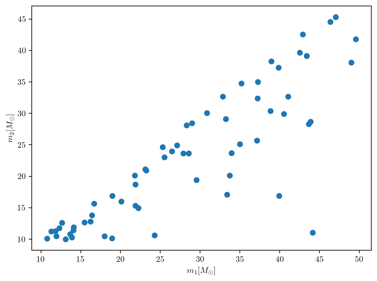
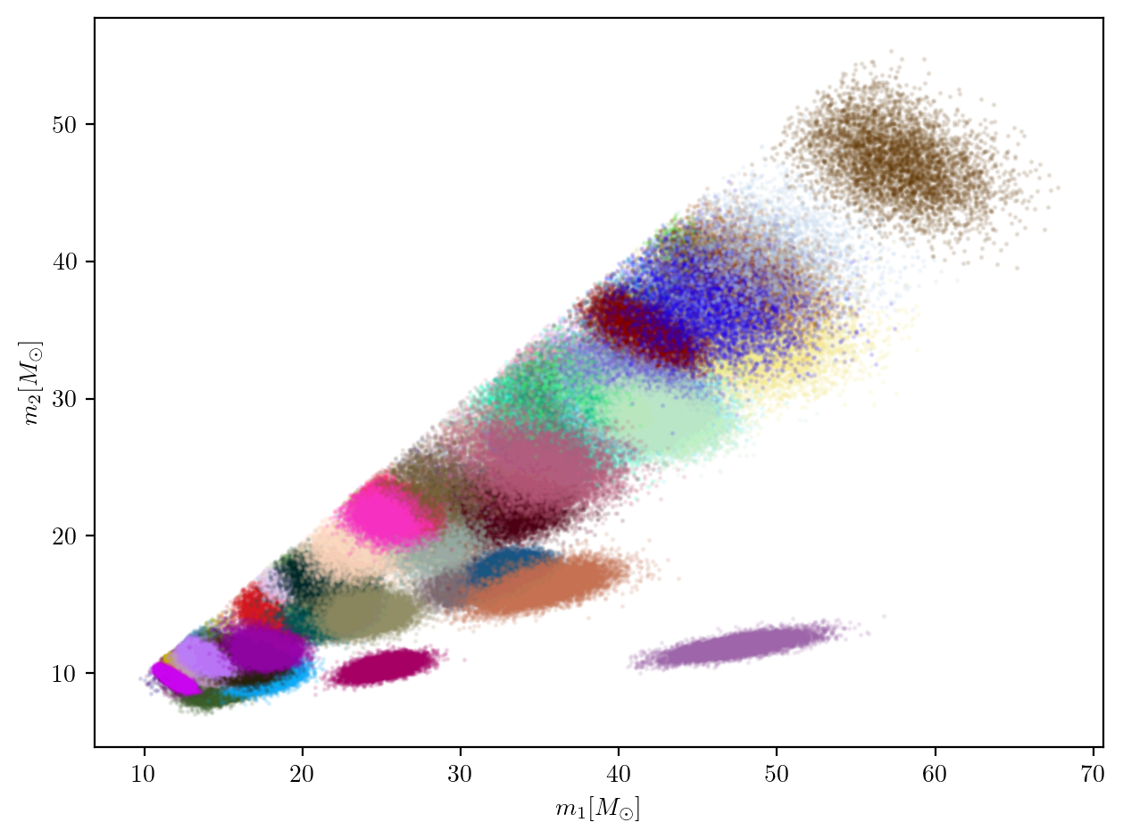
We can also visualize the injections and posterior samples. Below are two plots showing the injections and posterior samples in \(m_1\)-\(m_2\) plane.

---

All the code and files used in this tutorial can be found in hello-gwkokab/generating_mock_posterior_estimates.

References

[1]

M. Zeeshan and R. O'Shaughnessy. Eccentricity matters: impact of eccentricity on inferred binary black hole populations. Phys. Rev. D, 110:063009, Sep 2024. URL: https://link.aps.org/doi/10.1103/PhysRevD.110.063009, doi:10.1103/PhysRevD.110.063009.

[2]

Ilya Mandel, Will M. Farr, Andrea Colonna, Simon Stevenson, Peter Tiňo, and John Veitch. Model-independent inference on compact-binary observations. Monthly Notices of the Royal Astronomical Society, 465(3):3254–3260, 11 2016. URL: https://doi.org/10.1093/mnras/stw2883, arXiv:https://academic.oup.com/mnras/article-pdf/465/3/3254/8518218/stw2883.pdf, doi:10.1093/mnras/stw2883.

---

[1]

A niche model is a model that is specific to population inference of CBCs and not available in NumPyro.